17. Change We Can Believe In

LONG BEFORE I knew what calculus was, I sensed there was something special about it. My dad had spoken about it in reverential tones. He hadn't been able to go to college, being a child of the Depression, but somewhere along the line, maybe during his time in the South Pacific repairing B-24 bomber engines, he'd gotten a feel for what calculus could do. Imagine a mechanically controlled bank of antiaircraft guns automatically firing at an incoming fighter plane. Calculus, he supposed, could be used to tell the guns where to aim.

Define: reverential ˈrev.ɚ.əns 尊敬 Etymology: mid 16th cent.: from medieval Latin reverentialis, from the verb revereri from re- (expressing intensive force) + vereri ‘to fear’. 助记: re(加强) vereri(fear) 比较形似

Every year about a million American students take calculus. But far fewer really understand what the subject is about or could tell you why they were learning it. It's not their fault. There are so many techniques to master and so many new ideas to absorb that the overall framework is easy to miss.

Calculus is the mathematics of change.

It describes everything from the spread of epidemics to the zigs and zags of a well-thrown curveball. The subject is gargantuan—and so are its textbooks. Many exceed a thousand pages and work nicely as doorstops.

But within that bulk you'll find two ideas shining through. All the rest, as Rabbi Hillel said of the golden rule, is just commentary. Those two ideas are the derivative and the integral. Each dominates its own half of the subject, named, respectively, differential and integral calculus.

Roughly speaking, the derivative tells you how fast something is changing; the integral tells you how much it's accumulating. They were born in separate times and places: integrals in Greece around 250 B.C.; derivatives in England and Germany in the mid-1600s. Yet in a twist straight out of a Dickens novel, they've turned out to be blood relatives—though it took almost two millennia for anyone to see the family resemblance.

The next chapter will explore that astonishing connection, as well as the meaning of integrals. But first, to lay the groundwork, let's look at derivatives.

Derivatives are all around us, even if we don't recognize them as such. For example, the slope of a ramp is a derivative. Like all derivatives, it measures a rate of change—in this case, how far you're going up or down for every step you take. A steep ramp has a large derivative. A wheelchair-accessible ramp, with its gentle gradient, has a small derivative.

Every field has its own version of a derivative. Whether it goes by marginal return or growth rate or velocity or slope, a derivative by any other name still smells as sweet. Unfortunately, many students seem to come away from calculus with a much narrower interpretation, regarding the derivative as synonymous with the slope of a curve.

Their confusion is understandable. It's caused by our reliance on graphs to express quantitative relationships. By plotting y versus x to visualize how one variable affects another, all scientists translate their problems into the common language of mathematics. The rate of change that really concerns them—a viral growth rate, a jet's velocity, or whatever—then gets converted into something much more abstract but easier to picture: a slope on a graph.

Like slopes, derivatives can be positive, negative, or zero, indicating whether something is rising, falling, or leveling off. Consider Michael Jordan flying through the air before making one of his thunderous dunks.

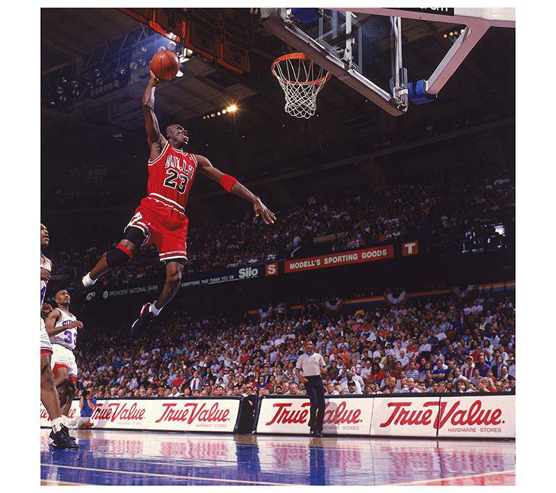
Just after liftoff, his vertical velocity (the rate at which his elevation changes in time and, thus, another derivative) is positive, because he's going up. His elevation is increasing. On the way down, this derivative is negative. And at the highest point of his jump, where he seems to hang in the air, his elevation is momentarily unchanging and his derivative is zero. In that sense he truly is hanging.

There's a more general principle at work here—things always change slowest at the top or the bottom. It's especially noticeable here in Ithaca. During the darkest depths of winter, the days are not just unmercifully short; they barely improve from one to the next. Whereas once spring starts popping, the days lengthen rapidly. All of this makes sense. Change is most sluggish at the extremes precisely because the derivative is zero there. Things stand still, momentarily.

This zero-derivative property of peaks and troughs underlies some of the most practical applications of calculus. It allows us to use derivatives to figure out where a function reaches its maximum or minimum, an issue that arises whenever we're looking for the best or cheapest or fastest way to do something.

My high-school calculus teacher, Mr. Joffray, had a knack for making such “max-min” questions come alive. One day he came bounding into class and began telling us about his hike through a snow-covered field. The wind had apparently blown a lot of snow across part of the field, blanketing it heavily and forcing him to walk much more slowly there, while the rest of the field was clear, allowing him to stride through it easily. In a situation like that, he wondered what path a hiker should take to get from point A to point B as quickly as possible.

Define: knack 诀窍 助记: knack - crack

One thought would be to {trudge} straight across the deep snow, to cut down on the slowest part of the hike. The downside, though, is the rest of the trip will take longer than it would otherwise.

 Another strategy is to head straight from A to B. That's certainly the shortest distance, but it does cost extra time in the most arduous part of the trip.

With differential calculus you can find the best path. It's a certain specific compromise between the two paths considered above.

The analysis involves four main steps. (For those who'd like to see the details, references are given in the notes on.

First, notice that the total time of travel—which is what we're trying to minimize—depends on where the hiker emerges from the snow. He could choose to emerge anywhere, so let's consider all his possible exit points as a variable. Each of these locations can be characterized succinctly by specifying a single number: the distance x where the hiker emerges from the snow.

(Implicitly, the travel time also depends on the locations of A and B and on the hiker's speeds in both parts of the field, but all those parameters are given. The only thing under the hiker's control is x.)

Second, given a choice of x and the known locations of the starting point A and the destination B, we can calculate how much time the hiker spends walking through the fast and slow parts of the field. For each leg of the trip, this calculation requires the Pythagorean theorem and the old algebra mantra “distance equals rate times time.” Adding the times for both legs together then yields a formula for the total travel time, T, as a function of x.

Third, we graph T versus x. The bottom of the curve is the point we're seeking—it corresponds to the least time of travel and hence the fastest trip.

Fourth, to find this lowest point, we invoke the zero-derivative principle mentioned above. We calculate the derivative of T, set it equal to zero, and solve for x.

These four steps require a command of geometry, algebra, and various derivative formulas from calculus—skills equivalent to fluency in a foreign language and, therefore, stumbling blocks for many students.

But the final answer is worth the struggle. It reveals that the fastest path obeys a relationship known as Snell's law. What's spooky is that nature obeys it too.

Snell's law describes how light rays bend when they pass from air into water, as they do when the sun shines into a swimming pool. Light moves more slowly in water, much like the hiker in the snow, and it bends accordingly to minimize its travel time. Similarly, light bends when it travels from air into glass or plastic, as when it refracts through your eyeglass lenses.

The eerie point is that light behaves as if it were considering all possible paths and then taking the best one. Nature—cue the theme from The Twilight Zone—somehow knows calculus.

18. It Slices, It Dices

MATHEMATICAL SIGNS AND symbols are often cryptic, but the best of them offer visual clues to their own meaning. The symbols for zero, one, and infinity aptly resemble an empty hole, a single mark, and an endless loop: 0, 1, ∞. And the equal sign, =, is formed by two parallel lines because, as its originator, Welsh mathematician Robert Recorde, wrote in 1557, “no two things can be more equal.”

In calculus the most recognizable icon is the integral sign:

Its graceful lines are evocative of a musical clef or a violin's f-hole—a fitting coincidence, given that some of the most enchanting harmonies in mathematics are expressed by integrals. But the real reason that the mathematician Gottfried Leibniz chose this symbol is much less poetic. It's simply a long-necked S, for “summation.”

As for what's being summed, that depends on context. In astronomy, the gravitational pull of the sun on the Earth is described by an integral. It represents the collective effect of all the minuscule forces generated by each solar atom at their varying distances from the Earth. In oncology, the growing mass of a solid tumor can be modeled by an integral. So can the cumulative amount of drug administered during the course of a chemotherapy regimen.

To understand why sums like these require integral calculus and not the ordinary kind of addition we learned in grade school, let's consider what challenges we'd face if we actually tried to calculate the sun's gravitational pull on the Earth. The first difficulty is that the sun is not a point . . . and neither is the Earth. Both of them are gigantic balls made up of stupendous numbers of atoms. Every atom in the sun exerts a gravitational tug on every atom in the Earth. Of course, since atoms are tiny, their mutual attractions are almost infinitesimally small, yet because there are almost infinitely many of them, in aggregate they can still amount to something. Somehow we have to add them all up.

But there's a second and more serious difficulty: Those pulls are different for different pairs of atoms. Some are stronger than others. Why? Because the strength of gravity changes with distance—the closer two things are, the more strongly they attract. The atoms on the far sides of the sun and the Earth feel the least attraction; those on the near sides feel the strongest; and those in between feel forces of middling strength. Integral calculus is needed to sum all those changing forces. Amazingly, it can be done—at least in the idealized limit where we treat the Earth and the sun as solid spheres composed of infinitely many points of continuous matter, each exerting an infinitesimal attraction on the others. As in all of calculus: infinity and limits to the rescue!

Historically, integrals arose first in geometry, in connection with the problem of finding the areas of curved shapes. As we saw in chapter 16, the area of a circle can be viewed as the sum of many thin pie slices. In the limit of infinitely many slices, each of which is infinitesimally thin, those slices could then be cunningly rearranged into a rectangle whose area was much easier to find. That was a typical use of integrals. They're all about taking something complicated and slicing and dicing it to make it easier to add up.

In a 3-D generalization of this method, Archimedes (and before him, Eudoxus, around 400 B.C.) calculated the volumes of various solid shapes by reimagining them as stacks of many wafers or disks, like a salami sliced thin. By computing the changing volumes of the varying slices and then ingeniously integrating them—adding them back together—they were able to deduce the volume of the original whole.

Today we still ask budding mathematicians and scientists to sharpen their skills at integration by applying them to these classic geometry problems. They're some of the hardest exercises we assign, and a lot of students hate them, but there's no surer way to hone the facility with integrals needed for advanced work in every quantitative discipline from physics to finance.

One such mind-bender concerns the volume of the solid common to two identical cylinders crossing at right angles, like stovepipes in a kitchen.

It takes an unusual gift of imagination to visualize this three-dimensional shape. So there's no shame in admitting defeat and looking for a way to make it more palpable. To do so, you can resort to a trick my high-school calculus teacher used—take a tin can and cut the top off with metal shears to form a cylindrical coring tool. Then core a large Idaho potato or a piece of Styrofoam from two mutually perpendicular directions. Inspect the resulting shape at your leisure.

Computer graphics now make it possible to visualize this shape more easily.

Remarkably, it has square cross-sections, even though it was created from round cylinders.

It's a stack of infinitely many layers, each a wafer-thin square, tapering from a large square in the middle to progressively smaller ones and finally to single points at the top and bottom.

Still, picturing the shape is merely the first step. What remains is to determine its volume, by tallying the volumes of all the separate slices. Archimedes managed to do this, but only by virtue of his astounding ingenuity. He used a mechanical method based on levers and centers of gravity, in effect weighing the shape in his mind by balancing it against others he already understood. The downside of his approach, besides the prohibitive brilliance it required, was that it applied to only a handful of shapes.

Conceptual roadblocks like this stumped the world's finest mathematicians for the next nineteen centuries . . . until the mid-1600s, when James Gregory, Isaac Barrow, Isaac Newton, and Gottfried Leibniz established what's now known as the fundamental theorem of calculus. It forged a powerful link between the two types of change being studied in calculus: the cumulative change represented by integrals, and the local rate of change represented by derivatives (the subject of chapter 17).

By exposing this connection, the fundamental theorem greatly expanded the universe of integrals that could be solved, and it reduced their calculation to grunt work. Nowadays computers can be programmed to use it—and so can students. With its help, even the stovepipe problem that was once a world-class challenge becomes an exercise within common reach. (For the details of Archimedes's approach as well as the modern one, consult the references in the notes on.)

Before calculus and the fundamental theorem came along, only the simplest kinds of net change could be analyzed. When something changes steadily, at a constant rate, algebra works beautifully. This is the domain of “distance equals rate times time.” For example, a car moving at an unchanging speed of 60 miles per hour will surely travel 60 miles in the first hour, and 120 miles by the end of the second hour.

But what about change that proceeds at a changing rate? Such changing change is all around us—in the accelerating descent of a penny dropped from a tall building, in the ebb and flow of the tides, in the elliptical orbits of the planets, in the circadian rhythms within us. Only calculus can cope with the cumulative effects of changes as non-uniform as these.

For nearly two millennia after Archimedes, just one method existed for predicting the net effect of changing change: add up the varying slices, bit by bit. You were supposed to treat the rate of change as constant within each slice, then invoke the analog of “distance equals rate times time” to inch forward to the end of that slice, and repeat until all the slices were dealt with. Most of the time it couldn't be done. The infinite sums were too hard.

The fundamental theorem enabled a lot of these problems to be solved—not all of them, but many more than before. It often gave a shortcut for solving integrals, at least for the elementary functions (sums and products of powers, exponentials, logarithms, and trig functions) that describe so many of the phenomena in the natural world.

Here's an analogy that I hope will shed some light on what the fundamental theorem says and why it's so helpful. (My colleague Charlie Peskin at New York University suggested it.) Imagine a staircase. The total change in height from the top to the bottom is the sum of the rises of all the steps in between. That's true even if some of the steps rise more than others and no matter how many steps there are.

The fundamental theorem of calculus says something similar for functions—if you integrate the derivative of a function from one point to another, you get the net change in the function between the two points. In this analogy, the function is like the elevation of each step compared to ground level. The rises of individual steps are like the derivative. Integrating the derivative is like summing the rises. And the two points are the top and the bottom.

Why is this so helpful? Suppose you're given a huge list of numbers to sum, as occurs whenever you're calculating an integral by slices. If you can somehow manage to find the corresponding staircase—in other words, if you can find an elevation function for which those numbers are the rises—then computing the integral is a snap. It's just the top minus the bottom.

That's the great speedup made possible by the fundamental theorem. And it's why we torture all beginning calculus students with months of learning how to find elevation functions, technically called antiderivatives or indefinite integrals. This advance allowed mathematicians to forecast events in a changing world with much greater precision than had ever been possible.

From this perspective, the lasting legacy of integral calculus is a Veg-O-Matic view of the universe. Newton and his successors discovered that nature itself unfolds in slices. Virtually all the laws of physics found in the past 300 years turned out to have this character, whether they describe the motions of particles or the flow of heat, electricity, air, or water. Together with the governing laws, the conditions in each slice of time or space determine what will happen in adjacent slices.

The implications were profound. For the first time in history, rational prediction became possible . . . not just one slice at a time but, with the help of the fundamental theorem, by leaps and bounds.

So we're long overdue to update our slogan for integrals—from “It slices, it dices” to “Recalculating. A better route is available.”

19. All about e

A FEW NUMBERS ARE SUCH CELEBRITIES that they go by single-letter stage names, something not even Madonna or Prince can match. The most famous is π, the number formerly known as 3.14159 . . .

Close behind is i, the it-number of algebra, the imaginary number so radical it changed what it meant to be a number. Next on the A list?

Say hello to e. Nicknamed for its breakout role in exponential growth, e is now the Zelig of advanced mathematics. It pops up everywhere, peeking out from the corners of the stage, teasing us by its presence in incongruous places. For example, along with the insights it offers about chain reactions and population booms, e has a thing or two to say about how many people you should date before settling down.

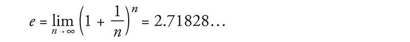
But before we get to that, what is e, exactly? Its numerical value is 2.71828 . . . but that's not terribly enlightening. I could tell you that e equals the limiting number approached by the sum

as we take more and more terms. But that's not particularly helpful either. Instead, let's look at e in action.

Imagine that you've deposited $1,000 in a savings account at a bank that pays an incredibly generous interest rate of 100 percent, compounded annually. A year later, your account would be worth $2,000—the initial deposit of $1,000 plus the 100 percent interest on it, equal to another $1,000.

Knowing a sucker when you see one, you ask the bank for even more favorable terms: How would they feel about compounding the interest semiannually, meaning that they'd be paying only 50 percent interest for the first six months, followed by another 50 percent for the second six months? You'd clearly do better than before—since you'd gain interest on the interest—but how much better?

The answer is that your initial $1,000 would grow by a factor of 1.50 over the first half of the year, and then by another factor of 1.50 over the second half. And since 1.50 times 1.50 is 2.25, your money would amount to a cool $2,250 after one year, substantially more than the $2,000 you got from the original deal.

What if you pushed even harder and persuaded the bank to divide the year into more and more periods—daily, by the second, or even by the nanosecond? Would you make a small fortune?

To make the numbers come out nicely, here's the result for a year divided into 100 equal periods, .after each of which you'd be paid 1 percent interest (the 100 percent annual rate divided evenly into 100 installments): your money would grow by a factor of 1.01 raised to the 100th power, and that comes out to be about 2.70481. In other words, instead of $2,000 or $2,250, you'd have $2,704.81.

Finally, the ultimate: if the interest was compounded infinitely often—this is called continuous compounding—your total after one year would be bigger still, but not by much: $2,718.28. The exact answer is $1,000 times e, where e is defined as the limiting number arising from this process:

This is a quintessential calculus argument. As we discussed in the last few chapters when we calculated the area of a circle or pondered the sun's gravitational pull on the Earth, what distinguishes calculus from the earlier parts of math is its willingness to confront—and harness—the awesome power of infinity. Whether we're looking at limits, derivatives, or integrals, we always have to sidle up to infinity in one way or another.

In the limiting process that led to e above, we imagined slicing a year into more and more compounding periods, windows of time that became thinner and thinner, ultimately approaching what can only be described as infinitely many, infinitesimally thin windows. (This might sound paradoxical, but it's really no worse than treating a circle as the limit of a regular polygon with more and more sides, each of which gets shorter and shorter.) The fascinating thing is that the more often the interest is compounded, the less your money grows during each period. Yet it still amounts to something substantial after a year, because it's been multiplied over so many periods!

This is a clue to the ubiquity of e. It often arises when something changes through the cumulative effect of many tiny events.

Consider a lump of uranium undergoing radioactive decay. Moment by moment, every atom has a certain small chance of disintegrating. Whether and when each one does is completely unpredictable, and each such event has an infinitesimal effect on the whole. Nevertheless, in ensemble these trillions of events produce a smooth, predictable, exponentially decaying level of radioactivity.

Or think about the world's population, which grows approximately exponentially. All around the world, children are being born at random times and places, while other people are dying, also at random times and places. Each event has a minuscule impact, percentagewise, on the world's overall population—yet in aggregate that population grows exponentially at a very predictable rate.

Another recipe for e combines randomness with enormous numbers of choices. Let me give you two examples inspired by everyday life, though in highly stylized form.

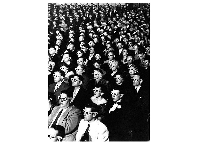
Imagine there's a very popular new movie showing at the local theater. It's a romantic comedy, and hundreds of couples (many more than the theater can accommodate) are lined up at the box office, desperate to get in. Once a lucky couple get their tickets, they scramble inside and choose two seats right next to each other. To keep things simple, let's suppose they choose these seats at random, wherever there's room. In other words, they don't care whether they sit close to the screen or far away, on the aisle or in the middle of a row. As long as they're together, side by side, they're happy.

Also, let's assume no couple will ever slide over to make room for another. Once a couple sits down, that's it. No courtesy whatsoever. Knowing this, the box office stops selling tickets as soon as there are only single seats left. Otherwise brawls would ensue.

At first, when the theater is pretty empty, there's no problem. Every couple can find two adjacent seats. But after a while, the only seats left are singles—solitary, uninhabitable dead spaces that a couple can't use. In real life, people often create these buffers deliberately, either for their coats or to avoid sharing an armrest with a repulsive stranger. In this model, however, these dead spaces just happen by chance.

The question is: When there's no room left for any more couples, what fraction of the theater's seats are unoccupied?

The answer, in the case of a theater with many seats per row, turns out to approach

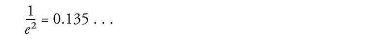
so about 13.5 percent of the seats go to waste.

Although the details of the calculation are too intricate to present here, it's easy to see that 13.5 percent is in the right ballpark by comparing it with two extreme cases. If all couples sat next to each other, packed in with perfect efficiency like sardines, there'd be no wasted seats.

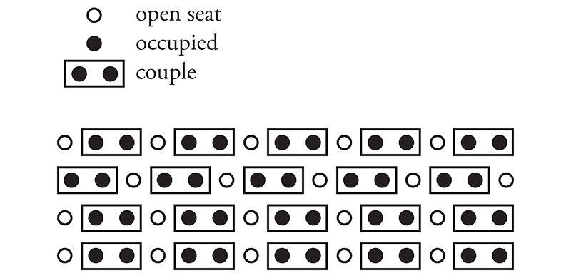
However, if they'd positioned themselves as inefficiently as possible, always with an empty seat between them (and leaving an empty aisle seat on one end or the other of each row, as in the diagram below), one-third of the seats would be wasted, because every couple uses three seats: two for themselves, and one for the dead space.

Guessing that the random case should lie somewhere between perfect efficiency and perfect inefficiency, and taking the average of 0 and , we'd expect that about , or 16.7 percent, of the seats would be wasted, not far from the exact answer of 13.5 percent.

Here the large number of choices came about because of all the ways that couples could be arranged in a huge theater. Our final example is also about arranging couples, except now in time, not space. What I'm referring to is the vexing problem of how many people you should date before choosing a mate. The real-life version of this problem is too hard for math, so let's consider a simplified model. Despite its unrealistic assumptions, it still captures some of the heartbreaking. uncertainties of romance.

Let's suppose you know how many potential mates you're going to meet during your lifetime. (The actual number is not important as long as it's known ahead of time and it's not too small.)

Also assume you could rank these people unambiguously if you could see them all at once. The tragedy, of course, is that you can't. You meet them one at a time, in random order. So you can never be sure if Dreamboat—who'd rank number 1 on your list—is just around the corner, or whether you've already met and parted.

And the way this game works is, once you let someone go, he or she is gone. No second chances.

Finally, assume you don't want to settle. If you end up with Second Best, or anyone else who, in retrospect, wouldn't have made the top of your list, you'll consider your love life a failure.

Is there any hope of choosing your one true love? If so, what can you do to give yourself the best odds?

A good strategy, though not the best one, is to divide your dating life into two equal halves. In the first half, you're just playing the field; in the second, you're ready to get serious, and you're going to grab the first person you meet who's better than everyone else you've dated so far.

With this strategy, there's at least a 25 percent chance of snagging Dreamboat. Here's why: You have a 50-50 chance of meeting Dreamboat in the second half of your dating life, your “get serious” phase, and a 50-50 chance of meeting Second Best in the first half, while you're playing the field. If both of those things happen—and there is a 25 percent chance that they will—then you'll end up with your one true love.

That's because Second Best raised the bar so high. No one you meet after you're ready to get serious will tempt you except Dreamboat. So even though you can't be sure at the time that Dreamboat is, in fact, The One, that's who he or she will turn out to be, since no one else can clear the bar set by Second Best.

The optimal strategy, however, is to stop playing the field a little sooner, after only 1/e, or about 37 percent, of your potential dating lifetime. That gives you a 1/e chance of ending up with Dreamboat.

As long as Dreamboat isn't playing the e game too.

20. Loves Me, Loves Me Not

“IN THE SPRING,” wrote Tennyson, “a young man's fancy lightly turns to thoughts of love.” Alas, his would-be partner has thoughts of her own—and the interplay between them can lead to the tumultuous ups and downs that make new love so thrilling, and so painful. To explain these swings, many lovelorn souls have sought answers in drink; others have turned to poetry. We'll consult calculus.

The analysis below is offered tongue-in-cheek, but it touches on a serious point: While the laws of the heart may elude us forever, the laws of inanimate things are now well understood. They take the form of differential equations, which describe how interlinked variables change from moment to moment, depending on their current values. As for what such equations have to do with romance—well, at the very least they might shed a little light on why, in the words of another poet, “the course of true love never did run smooth.”

To illustrate the approach, suppose Romeo is in love with Juliet but that, in our version of the story, Juliet is a fickle lover. The more Romeo loves her, the more she wants to run away and hide. But when he takes the hint and backs off, she begins to find him strangely attractive. He, however, tends to mirror her: he warms up when she loves him and cools down when she hates him.

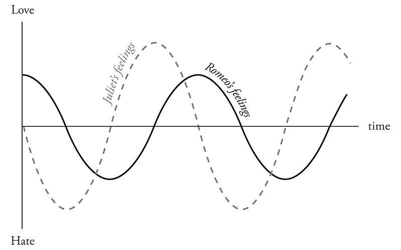
What happens to our star-crossed lovers? How does their love ebb and flow over time? That's where calculus comes in. By writing equations that summarize how Romeo and Juliet respond to each other's affections and then solving those equations with calculus, we can predict the course of their affair. The resulting forecast for this couple is, tragically, a never-ending cycle of love and hate. At least they manage to achieve simultaneous love a quarter of the time.

To reach this conclusion, I've assumed that Romeo's behavior can be modeled by the differential equation

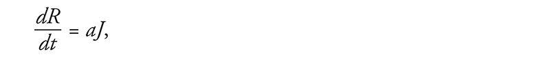
which describes how his love (represented by R) changes in the next instant (represented by dt). According to this equation, the amount of change (dR) is just a multiple (a) of Juliet's current love (J) for him. This reflects what we already know—that Romeo's love goes up when Juliet loves him—but it assumes something much stronger. It says that Romeo's love increases in direct linear proportion to how much Juliet loves him. This assumption of linearity is not emotionally realistic, but it makes the equations much easier to solve.

Juliet's behavior, by contrast, can be modeled by the equation

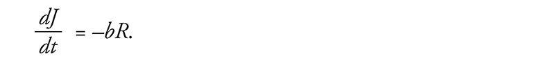
The negative sign in front of the constant b reflects her tendency to cool off when Romeo is hot for her.

The only remaining thing we need to know is how the lovers felt about each other initially (R and J at time t = 0). Then everything about their affair is predetermined. We can use a computer to inch R and J forward, instant by instant, changing their values as prescribed by the differential equations. Actually, with the help of the fundamental theorem of calculus, we can do much better than that. Because the model is so simple, we don't have to trudge forward one moment at a time. Calculus yields a pair of comprehensive formulas that tell us how much Romeo and Juliet will love (or hate) each other at any future time.

The differential equations above should be recognizable to students of physics: Romeo and Juliet behave like simple harmonic oscillators. So the model predicts that R/(t) and J/(t)—the functions that describe the time course of their relationship—will be sine waves, each waxing and waning but peaking at different times.

The model can be made more realistic in various ways. For instance, Romeo might react to his own feelings as well as to Juliet's. He might be the type of guy who is so worried about throwing himself at her that he slows himself down as his love for her grows. Or he might be the other type, one who loves feeling in love so much that he loves her all the more for it.

Add to those possibilities the two ways Romeo could react to Juliet's affections—either increasing or decreasing his own—and you see that there are four personality types, each corresponding to a different romantic style. My students and those in Peter Christopher's class at Worcester Polytechnic Institute have suggested such descriptive names as Hermit and Malevolent Misanthrope for the particular kind of Romeo who damps down his own love and also recoils from Juliet's. Whereas the sort of Romeo who gets pumped by his own ardor but turned off by Juliet's has been called Narcissistic Nerd, Better Latent Than Never, and a Flirting Fink. (Feel free to come up with your own names for these two types and the other two possibilities.)

Although these examples are whimsical, the kinds of equations that arise in them are profound. They represent the most powerful tool humanity has ever created for making sense of the material world. Sir Isaac Newton used differential equations to solve the ancient mystery of planetary motion. In so doing, he unified the earthly and celestial spheres, showing that the same laws of motion applied to both.

In the nearly 350 years since Newton, mankind has come to realize that the laws of physics are always expressed in the language of differential equations. This is true for the equations governing the flow of heat, air, and water; for the laws of electricity and magnetism; even for the unfamiliar and often counterintuitive atomic realm, where quantum mechanics reigns.

In all cases, the business of theoretical physics boils down to finding the right differential equations and solving them. When Newton discovered this key to the secrets of the universe, he felt it was so precious that he published it only as an anagram in Latin. Loosely translated, it reads: “It is useful to solve differential equations.”

The silly idea that love affairs might likewise be described by differential equations occurred to me when I was in love for the first time, trying to understand my girlfriend's baffling behavior. It was a summer romance at the end of my sophomore year in college. I was a lot like the first Romeo above, and she was even more like the first Juliet. The cycling of our relationship drove me crazy until I realized that we were both acting mechanically, following simple rules of push and pull. But by the end of the summer my equations started to break down, and I was more mystified than ever. As it turned out, there was an important variable that I'd left out of the equations—her old boyfriend wanted her back.

In mathematics we call this a three-body problem. It's notoriously intractable, especially in the astronomical context where it first arose. After Newton solved the differential equations for the two-body problem (thus explaining why the planets move in elliptical orbits around the sun), he turned his attention to the three-body problem for the sun, Earth, and moon. He couldn't solve it, and neither could anyone else. It later turned out that the three-body problem contained the seeds of chaos, rendering its behavior unpredictable in the long run.

Newton knew nothing about chaotic dynamics, but according to his friend Edmund Halley, he complained that the three-body problem had “made his head ache, and kept him awake so often, that he would think of it no more.”

I'm with you there, Sir Isaac.

21. Step Into the Light

MR. DICURCIO WAS my mentor in high school. He was disagreeable and demanding, with nerdy black-rimmed glasses and a penchant for sarcasm, so his charms were easy to miss. But I found his passion for physics irresistible.

One day I mentioned to him that I was reading a biography of Einstein. The book said that as a college student, Einstein had been dazzled by something called Maxwell's equations for electricity and magnetism, and I said I couldn't wait until I knew enough math to learn what they were.

This being a boarding school, we were eating dinner together at a big table with several other students, his wife, and his two daughters, and Mr. DiCurcio was serving mashed potatoes. At the mention of Maxwell's equations, he dropped the serving spoon, grabbed a paper napkin, and began writing lines of cryptic symbols—dots and crosses, upside-down triangles, /E/s and /B/s with arrows over them—and suddenly he seemed to be speaking in tongues: “The curl of a curl is grad div minus del squared . . .”

That abracadabra he was mumbling? I realize now he was speaking in vector calculus, the branch of math that describes the invisible fields all around us. Think of the magnetic field that twists a compass needle northward, or the gravitational field that pulls your chair to the floor, or the microwave field that nukes your dinner.

twilight realm where math meets reality. Indeed, the story of James Clerk Maxwell and his equations offers one of the eeriest instances of the unreasonable effectiveness of mathematics. Somehow, by shuffling a few symbols, Maxwell discovered what light is.

To give a sense of what Maxwell accomplished and, more generally, what vector calculus is about, let's begin with the word “vector.” It comes from the Latin root vehere, “to carry,” which also gives us words like “vehicle” and “conveyor belt.” To an epidemiologist, a vector is the carrier of a pathogen, like the mosquito that conveys malaria to your bloodstream. To a mathematician, a vector (at least in its simplest form) is a step that carries you from one place to another.

Think about one of those diagrams for aspiring ballroom dancers covered with arrows indicating how to move the right foot, then the left foot, as when doing the rumba:

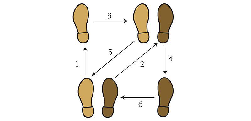
These arrows are vectors. They show two kinds of information: a direction (which way to move that foot) and a magnitude (how far to move it). All vectors do that same double duty.

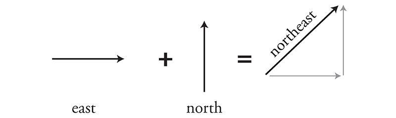
Vectors can be added and subtracted, just like numbers, except their directionality makes things a little trickier. Still, the right way to add vectors becomes clear if you think of them as dance instructions. For example, what do you get when you take one step east followed by one step north? A vector that points northeast, naturally.

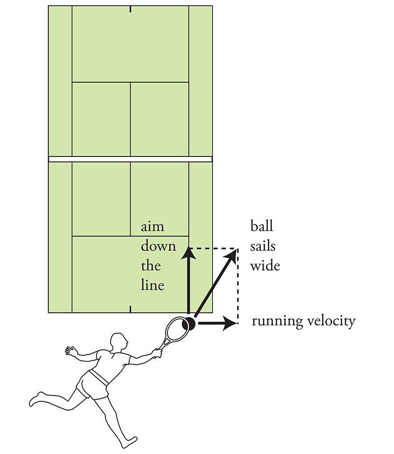
Remarkably, velocities and forces work the same way—they too add just like dance steps. This should be familiar to any tennis player who's ever tried to imitate Pete Sampras and hit a forehand down the line while sprinting at full speed toward the sideline. If you naively aim your shot where you want it to go, it will sail wide because you forgot to take your own running into account. The ball's velocity relative to the court is the sum of two vectors: the ball's velocity relative to you (a vector pointing down the line, as intended), and your velocity relative to the court (a vector pointing sideways, since that's the direction you're running). To hit the ball where you want it to go, you have to aim slightly crosscourt, to compensate for your sideways motion.

Beyond such vector algebra lies vector calculus, the kind of math Mr. DiCurcio was using. Calculus, you'll recall, is the mathematics of change. And so whatever vector calculus is, it must involve vectors that change, either from moment to moment or from place to place. In the latter case, one speaks of a “vector field.”

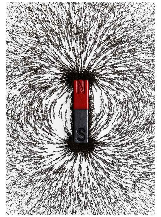
A classic example is the force field around a magnet. To visualize it, put a magnet on a piece of paper and sprinkle iron filings everywhere. Each filing acts like a little compass needle—it aligns with the direction of local “north,” determined by the magnetic field at that point. Viewed in aggregate, these filings reveal a spectacular pattern of magnetic-field lines leading from one pole of the magnet to the other.

The direction and magnitude of the vectors in a magnetic field vary from point to point. As in all of calculus, the key tool for quantifying such changes is the derivative. In vector calculus the derivative operator goes by the name of del, which has a folksy southern ring to it, though it actually alludes to the Greek letter ∆ (delta), commonly used to denote a change in some variable. As a reminder of that kinship, “del” is written like this: ∇. (That was the mysterious upside-down triangle Mr. DiCurcio kept writing on the napkin.)

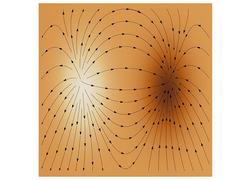
It turns out there are two different but equally natural ways to take the derivative of a vector field by applying del to it. The first gives what's known as the field's divergence (the “div” that Mr. DiCurcio muttered). To get an intuitive feeling for what the divergence measures, take a look at the vector field below, which shows how water would flow from a source on the left to a sink on the right.

For this example, instead of using iron filings to track the vector field, imagine lots of tiny corks or bits of leaves floating on the water surface. We're going to use them as probes. Their motion will tell us how the water is moving at each point. Specifically, imagine what would happen if we put a small circle of corks around the source. Obviously, the corks would spread apart and the circle would expand, because water flows away from a source. It diverges there. And the stronger the divergence, the faster the area of our cork-circle would grow. That's what the divergence of a vector field measures: how fast the area of a small circle of corks grows.

The image below shows the numerical value of the divergence at each point in the field we've just been looking at, coded by shades of gray. Lighter shades show points where the flow has a positive divergence. Darker shades show places of negative divergence, meaning that the flow would compress a tiny cork-circle centered there.

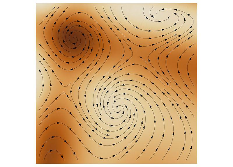
The other kind of derivative measures the curl of a vector field. Roughly speaking, it indicates how strongly the field is swirling about a given point. (Think of the weather maps you've seen on the local news showing the rotating wind patterns around hurricanes or tropical storms.) In the vector field below, regions that look like hurricanes have a large curl.

By embellishing the vector field with shading, we can now show where the curl is most positive (lightest regions) and most negative (darkest regions). Notice that this also tells us whether the flow is spinning counterclockwise or clockwise.

The curl is extremely informative for scientists working in fluid mechanics and aerodynamics. A few years ago my colleague Jane Wang used a computer to simulate the pattern of airflow around a dragonfly as it hovered in place. By calculating the curl, she found that when a dragonfly flaps its wings, it creates pairs of counter-rotating vortices that act like little tornadoes beneath its wings, producing enough lift to keep the insect aloft. In this way, vector calculus is helping to explain how dragonflies, bumblebees, and hummingbirds can fly—something that had long been a mystery to conventional fixed-wing aerodynamics.

With the notions of divergence and curl in hand, we're now ready to revisit Maxwell's equations. They express four fundamental laws: one for the divergence of the electric field, another for its curl, and two more of the same type but now for the magnetic field. The divergence equations relate the electric and magnetic fields to their sources, the charged particles and currents that produce them in the first place. The curl equations describe how the electric and magnetic fields interact and change over time. In so doing, these equations express a beautiful symmetry: they link one field's rate of change in time to the other field's rate of change in space, as quantified by its curl.

Using mathematical maneuvers equivalent to vector calculus—which wasn't known in his day—Maxwell then extracted the logical consequences of those four equations. His symbol shuffling led him to the conclusion that electric and magnetic fields could propagate as a wave, somewhat like a ripple on a pond, except that these two fields were more like symbiotic organisms. Each sustained the other. The electric field's undulations re-created the magnetic field, which in turn re-created the electric field, and so on, with each pulling the other forward, something neither could do on its own.

That was the first breakthrough—the theoretical prediction of electromagnetic waves. But the real stunner came next. When Maxwell calculated the speed of these hypothetical waves, using known properties of electricity and magnetism, his equations told him that they traveled at about 193,000 miles per second—the same rate as the speed of light measured by the French physicist Hippolyte Fizeau a decade earlier!

How I wish I could have witnessed the moment when a human being first understood the true nature of light. By identifying it with an electromagnetic wave, Maxwell unified three ancient and seemingly unrelated phenomena: electricity, magnetism, and light. Although experimenters like Faraday and Ampère had previously found key pieces of this puzzle, it was only Maxwell, armed with his mathematics, who put them all together.

Today we are awash in Maxwell's once-hypothetical waves: Radio. Television. Cell phones. Wi-Fi. These are the legacy of his conjuring with symbols.